scipy.integrate.solve_ivpについて浅く掘る

2021-08-10

scipy.integrate.solve_ivpの実装について簡単に見ていきます。 Solving Ordinary Differential Equations I [1]と実際のコード[2]を参考にしています。

設定

今回はLorenz方程式を使用します。

Deterministic Nonperiodic Flow

$ \begin{cases} \dot{x}=\sigma(y-x)\\ \dot{y}=rx-y-xz\\ \dot{x}=xy-bz \end{cases} $

パラメータは代表的な$\sigma=10,b=8/3,r=28$を使います。

def lorenz(t, u, p=10, b=8/3, r=28):
    x, y, z = u

    dxdt = -p * x + p * y
    dydt = -x * z + r * x - y
    dzdt =  x * y - b * z

    return np.array([dxdt, dydt, dzdt])

今回は初期値を$(0.1, 0.1, 0.1)$とし、時間$t=0$から$t=40$で解いていきます。


使うライブラリは以下の通りです。

import matplotlib.pyplot as plt
import numpy as np
from scipy.integrate import solve_ivp

solve_ivp

scipy.integrate.solve_ivpを使って解いていきます。

def solve_ivp(
    fun, t_span, y0, method='RK45', t_eval=None, dense_output=False,
    events=None, vectorized=False, args=None, **options
):

方程式を解く際にscipy.integrate.odeintscipy.integrate.odeを使っている例が多いですが、現在はOld APIに指定されています。 Integration and ODEs | Old API


対象の方程式、時間のスパン、初期値を与え、解きます。

sol = solve_ivp(lorenz, (0,40), [0.1, 0.1, 0.1])

計算結果はOdeResultというオブジェクトで返ってきます。これは結局dictみたいなものです。[*1]

OdeResult(t=ts, y=ys, 
          sol=sol, t_events=t_events, y_events=y_events,
          fev=solver.nfev, njev=solver.njev, nlu=solver.nlu,
          status=status, message=message, success=status >= 0)

軌道はyに格納されていて、次元×STEP数のnp.ndarrayです。

3次元プロットをすることで軌道を確認します。

fig, ax = plt.subplots(subplot_kw=dict(projection='3d'))
ax.plot(*list(sol.y))
plt.show()

Lorenz atractor

アトラクターを確認することができました。

method=

scipy.integrate.solve_ivpではOdeSolverを使用して計算を行なっています。

solverは引数methodで設定されます。デフォルトではRK45が採用されています。

RK45はEmbedded Runge-Kutta Formulasの一つで、刻み幅の自動調整が行われています。

刻み幅hの推移を見ることで調整しているかどうかを確認します。
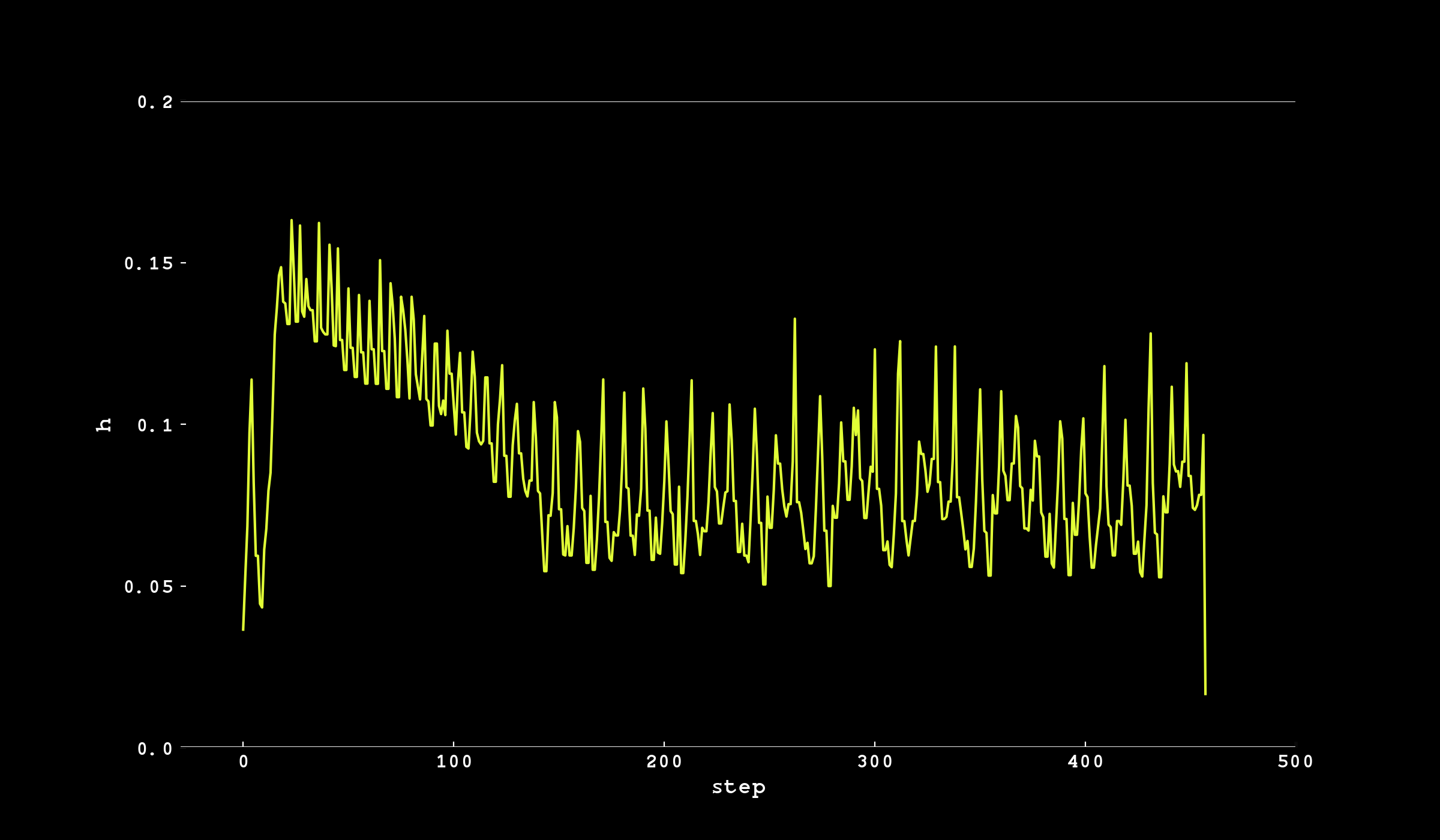
plt.plot(np.diff(sol.t))
plt.show()

h

刻み幅の動的更新が確認できます。


Embedded Runge-Kutta

Embedded Runge-Kutta(埋め込みルンゲ・クッタ)では $p$ 次の $b$ と、 $\hat{p}$ 次( $\hat{p}=p-1 \ or \ \hat{p}=p+1$ )の $\hat{b}$ を利用して計算を行います。

Butcher tableauは以下のようになります。

$$$ \def\arraystretch{1.5} \begin{array}{c|c} 0 & & & \\ c_1 & a_{21} & & & \\ c_2 & a_{31} & a_{32} & & \\ \vdots & \vdots & \vdots & \ddots & & \\ c_s & a_{s1} & a_{s2} & \cdots & a_{s, s-1} & \\ \hline & b_1 & b_2 & \cdots & b_{s-1} & b_s \\ \hline \\ & \hat{b_1} & \hat{b_2} & \cdots & \hat{b_{s-1}} & \hat{b_s} \\ \end{array} $$$

$ k_s =f(t_0+c_sh, y_0+h(a_{s1}k_1+...+a_{s, s-1}k_{s-1})) $


$p$次の$y_1$を計算します。

$ y_1 = y_0 + h(b_1k_1+...+b_sk_s) $

$\hat{p}$次の$\hat{y}_1$を計算します。

$ \hat{y}_1 = y_0 + h(\hat{b}_1k_1+...+\hat{b}_sk_s) $

solve_ivpはこの差 $y_1 - \hat{y}_1$ を$sc_i$以下に保ちます。

$ |y_{1i}-\hat{y_{1i}}|\leq sc_i \\ sc_i=Atol_i + max(|y_{0i}|,|y_{1i}|) Rtol_i $

rtol=1e-3, atol=1e-6とデフォルトで設定されています。

# scipy/integrate/_ivp/rk.py

class RungeKutta(OdeSolver):
    ...
    def _step_impl(self):

        ...
        scale = atol + np.maximum(np.abs(y), np.abs(y_new)) * rtol
        ...

$Rtol$と$Atol$を使用して、相対許容誤差と絶対許容誤差を制御できる。らしいです。

確かに、$Rtol$と$Atol$を小さくすることで$sc_i$を小さくできるので、誤差を小さくすることは可能です。

ただ、値の設定に関してちゃんとした物を発見できていないのでそのうち追記します。


$sc_i$を使用した$err$を元に刻み幅hを決定します。

$ err = \sqrt{\frac{1}{n}\displaystyle\sum_{i=1}^n({\frac{y_{1i}-\hat{y}_{1i}}{sc_i}})^2} $


RK45

C,A,Bに上記の記号$\bold{c}, \bold{a}, \bold{b}$が割り当てられています。Eは$\bold{\hat{b}}$に当たります。

こちらの値は以下の論文の値を参考にしていました。

Some Practical Runge-Kutta Formulas

class RK45(RungeKutta):
    ...

    C = np.array([0, 1/5, 3/10, 4/5, 8/9, 1])
    A = np.array([
        [0, 0, 0, 0, 0],
        [1/5, 0, 0, 0, 0],
        [3/40, 9/40, 0, 0, 0],
        [44/45, -56/15, 32/9, 0, 0],
        [19372/6561, -25360/2187, 64448/6561, -212/729, 0],
        [9017/3168, -355/33, 46732/5247, 49/176, -5103/18656]
    ])
    B = np.array([35/384, 0, 500/1113, 125/192, -2187/6784, 11/84])
    E = np.array([-71/57600, 0, 71/16695, -71/1920, 17253/339200, -22/525, 1/40])
    ...

刻み幅を指定する

刻み幅を指定する場合はt_evalを渡します。

例えば刻み幅0.01で計算を行いたい場合は以下のようになります。

(np.linspaceを使用していますが、np.arange(0.0, 40.01, 0.01)でも大丈夫です。)

sol = solve_ivp(
      lorenz, (0,40), [0.1, 0.1, 0.1],
      t_eval=np.linspace(0, 40, 4000)  # <- 追加
)

実装を簡単に確認します。

(1) まずt_evalを指定することでnp.searchsortedを使用してt_evalからt_eval_stepとして抽出します。

def solve_ivp(...):
    ...

    status = None
    while status is None:
       if t_eval is None:
           ts.append(t)
           ys.append(y)
       else:
           if solver.direction > 0:
               t_eval_i_new = np.searchsorted(t_eval, t, side='right')  # <- (1)
               t_eval_step = t_eval[t_eval_i:t_eval_i_new]
           else:
               ...

       if t_eval_step.size > 0:
           if sol is None:
               sol = solver.dense_output()
           ts.append(t_eval_step)
           ys.append(sol(t_eval_step))  # <- (2)
           t_eval_i = t_eval_i_new

(2) t_eval_stepPを使用して補間sol(t_eval_step)*2が行われます。 これによりt_evalにおける軌道が計算されます。

(補間についてはそのうち調べます。)

参考文献

Solving Ordinary Differential Equations I

book1

日本語訳も存在しますが、すでに販売を終了しており、図書館の貸し出し状態は不明だったのでこれを参考にしています。

II.1 THe First Runge-Kutta Methods

II.4 Practical Error Estimation and Step Size Selection


scipy.integrate.solve_ivp

scipy.integrate.solve_ivp | SciPy documentation

おまけ

OdeResult

scipy.solve_ivpの返り値であるOdeResultを確認します。

# scipy/integrate/_ivp/ivp.py

class OdeResult(OptimizeResult):
    pass
# scipy/optimize/optimize.py

class OptimizeResult(dict):
    """ Represents the optimization result.
      ...
    """

    def __getattr__(self, name):
        try:
            return self[name]
        except KeyError as e:
            raise AttributeError(name) from e

    __setattr__ = dict.__setitem__
    __delattr__ = dict.__delitem__

    def __repr__(self):
        if self.keys():
            m = max(map(len, list(self.keys()))) + 1
            return '\n'.join([k.rjust(m) + ': ' + repr(v)
                              for k, v in sorted(self.items())])
        else:
            return self.__class__.__name__ + "()"

    def __dir__(self):
        return list(self.keys())

sol(t_eval_step)

RkDenseOutput(...)(t_eval_step)は結局RkDenseOutput(...)._call_impl(t_eval_step)です。

# scipy/integrate/_ivp/rk.py

class RK45(RungeKutta):
    ...

    P = np.array(...)  # <-

class RungeKutta(OdeSolver):
    ...

    def _dense_output_impl(self):
        Q = self.K.T.dot(self.P)
        return RkDenseOutput(self.t_old, self.t, self.y_old, Q)

class RkDenseOutput(DenseOutput):
    def __init__(self, t_old, t, y_old, Q):
        ...

    def _call_impl(self, t): # <- 補間処理部分
        x = (t - self.t_old) / self.h
        if t.ndim == 0:
            p = np.tile(x, self.order + 1)
            p = np.cumprod(p)
        else:
            p = np.tile(x, (self.order + 1, 1))
            p = np.cumprod(p, axis=0)
        y = self.h * np.dot(self.Q, p)
        if y.ndim == 2:
            y += self.y_old[:, None]
        else:
            y += self.y_old

        return y
# scipy/integrate/_ivp/base.py

class DenseOutput(object):
    ...

    def __call__(self, t):
        ...

        return self._call_impl(t)  # <- 結局ここ

    ...